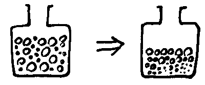
Motivation behind Simulated Annealing:

• Observation of metal cooled at a controlled temperature:
  • Slowly falling temperature allows the atoms in the molten metal to line themselves up and form a regular crystalline strucutre that has high density and low energy.
  • Abruptly falling temperature does not allow the atoms to orient themselves and results in a more amorphous material with low density and high energy.
• An analogy:

  An analogy to SA: shaking a bottle to increase its content's density.

• Can we emulate the thermodynamical process with today's fast computers?

Basic Terms of SA:

• Objective function: An objective function maps an input vector into a scalar E:

  

  where each is viewed as a point in an input space. The task of SA is to sample the input space effectively to find an that minimizes E.

• Move sets: The set of legal points available for exploration after x.
• Generating function: A generating function specifies the probability density function of the difference between the current point and the next point to be visited. Specifically, () is a random variable with probability density function , where T is the temperature. For common SA (especially when used in combinatorial optimization applications), is usually a function independent of the temperature T. Acceptance function: After a new point has been evaluated, SA decides whether to accept or reject it based on the value of an acceptance function . The most frequently used acceptance function is the Boltzmann probability distribution:

  

  where c is a system-dependent constant, T is the temperature, and is the energy difference between and :

  

  The common practice is to accept with probability . Note that when is negative, SA tends to accept the new point because it reduces the energy. When is positive, SA may accept the new point and end up in a higher energy state. In other words, SA can go either uphill or downhill; but the lower the temperature, the less likely SA is to accept any significant uphill actions.

• Annealing schedule: An annealing schedule regulates how rapidly the temperature T goes from high to low values, as a function of time or iteration counts. The exact interpretation of high and low and the specification of a good annealing schedule require certain problem-specific physical insights and/or trial-and-error. The easiest way of setting an annealing schedule is to decrease the temperature T by a certain percentage at each iteration.

SA Flowchart:

Step 1:

Choose a start point and set a high starting temperature T. Set the iteration count k to 1.

Step 2:

Evaluate the objective function:

Step 3:

Select with probability determined by the generating function . Set the new point equal to . (In conventional SA, also known as Boltzmann machines, the generating function is a Gaussian probability density function:

where () is the deviation of the new point from the current one, T is the temperature, and n is the dimension of the space under exploration.)

Step 4:

Calculate the new value of the objective function:

Step 5:

Set to and E to with probability determined by the acceptance function , where .

Step 6:

Reduce the temperature T according to the annealing schedule (usually by simply setting T equal to , where is a constant between 0 and 1).

Step 7:

Increment iteration count k. If k reaches the maximum iteration count, stop the iterating. Otherwise, go back to step 3.

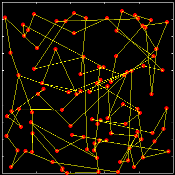
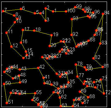
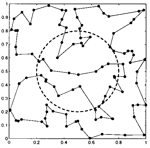
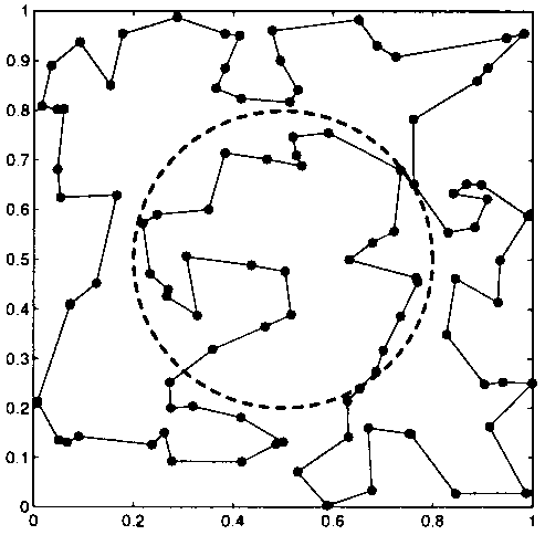
SA for Discrete (Combinatorial) Optimization: An Example:

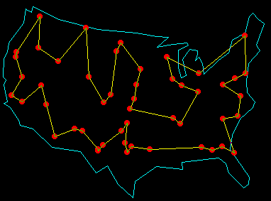
Travel Salesperson problem (TSP): how to transverse n cities once and only once with the minimal total distance?

Travel salesperson problem

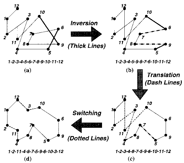
Three possible types of move sets for travel salesperson problem

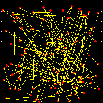
Initial random path	A path during SA process	Final path after SA process

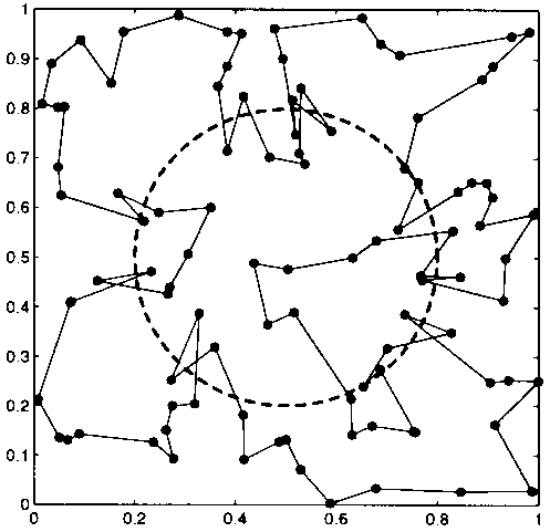
Cost of cross the circle = 0	Cost of cross the circle = 0.5	Cost of cross the circle = -0.3

Advantages of SAs:

• Derivative freeness (derivatives of the peaks function).
• For both continuous and discrete (combinatorial) optimization
• stochastic and less likely to get trapped in local minima
• No overhead of encoding and decoding
• Flexibility

Weakness of SA:

• Slowness
• Good move set schemes are somewhat non-intuitive for a given task.
• Cooling schedule is usually obtained by trial and error.

Reported SA Applications:

• VLSI design: placement and routing
• Neural networks and fuzzy modeling
• And many, many others.

Reference: Neuro-Fuzzy and Soft Computing