 |
rbfn.m
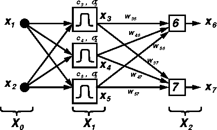
For simplicity, suppose that we are dealing with a 2-3-2
radial basis function network, and we have
100 input-output data pairs as the training data set.
The training data set can be represented by a
![]() matrix:
matrix:
![\begin{displaymath}
\left[
\begin{array}
{cccc}
x_{1,1} & x_{2,1} & t_{6,1} & t_...
...,100} & x_{2,100} & t_{6,100} & t_{7,100} \\ \end{array}\right]\end{displaymath}](img3.gif)
![\begin{displaymath}
{\bf X}_0 =
\left[
\begin{array}
{cc}
x_{1,1} & x_{2,1} \\ \...
... \vdots & \vdots \\ x_{1,100} & x_{2,100} \\ \end{array}\right]\end{displaymath}](img5.gif)
![\begin{displaymath}
{\bf T}=
\left[
\begin{array}
{cc}
t_{6,1} & t_{7,1} \\ \vdo...
... \vdots & \vdots \\ t_{6,100} & t_{7,100} \\ \end{array}\right]\end{displaymath}](img7.gif)
For discussion convenience, we shall also defined ![]() and
and ![]() as the node outputs for layer 1 and 2, respectively:
as the node outputs for layer 1 and 2, respectively:
![\begin{displaymath}
{\bf X}_1 =
\left[
\begin{array}
{ccc}
x_{3,1} & x_{4,1} & ...
...dots \\ x_{3,100} & x_{4,100} & x_{5,100} \\ \end{array}\right]\end{displaymath}](img10.gif)
![\begin{displaymath}
{\bf X}_2 =
\left[
\begin{array}
{cc}
x_{6,1} & x_{7,1} \\ ...
... \vdots & \vdots \\ x_{6,100} & x_{7,100} \\ \end{array}\right]\end{displaymath}](img11.gif)
The centers of the Gaussian functions in the second layer can be expressed as
![\begin{displaymath}
{\bf C}=
\left[
\begin{array}
{cc}
c_{11} & c_{12} \\
c_{21} & c_{22} \\
c_{31} & c_{32} \\ \end{array}\right],\end{displaymath}](img12.gif)
![\begin{displaymath}
{\bf C}=
\left[
\begin{array}
{c}
\sigma_1 \\
\sigma_2 \\
\sigma_3 \\ \end{array}\right],\end{displaymath}](img13.gif)
The parameters ![]() for the second layer can be defined as follows:
for the second layer can be defined as follows:
![\begin{displaymath}
{\bf W}=
\left[
\begin{array}
{cc}
w_{36} & w_{37} \\
w_{46} & w_{47} \\
w_{56} & w_{57} \\ \end{array}\right]\end{displaymath}](img15.gif)
The equations for computing the output of the first layer are
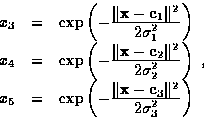
![\begin{displaymath}
{\bf X}_1 =
\left[
\begin{array}
{ccc}
x_{3,1} & x_{4,1} & ...
...\Vert^2}{\textstyle 2\sigma_3^2} \\ \end{array}\right]
\right),\end{displaymath}](img19.gif)
![\begin{displaymath}
{\bf X}_1 =
\exp \left(
\left[
\begin{array}
{ccc}
\Vert{\b...
...xtstyle 1}{\textstyle 2\sigma_3} \\ \end{array}\right]
\right)\end{displaymath}](img21.gif)
rbfn.m:
X1 = \exp(-(dist.^2)*diag(1./(2*SIGMA.^2)));
dist is the The equations for computing the output of the second layer are
![]()
![\begin{displaymath}[x_6 \; x_7]
=
[x_3 \; x_4 \; x_5]
*
\left[
\begin{array}
{cc...
...37} \\ w_{46} & w_{47} \\ w_{56} & w_{57} \\ \end{array}\right]\end{displaymath}](img24.gif)
![\begin{displaymath}
\left[
\begin{array}
{cc}
x_{6,1} & x_{7,1} \\ \vdots & \vdo...
...7} \\ w_{46} & w_{47} \\ w_{56} & w_{57} \\ \end{array}\right],\end{displaymath}](img25.gif)
![]()
rbfn.m:
X2 = X1*W;
The instantaneous error measure for the pth data pair is defined by
Ep = (t6,p-x6,p)2 + (t7,p-x7,p)2,
where t6,p and t7,p are the pth target outputs; x6,p and x7,p are the pth network outputs. The derivative of the above instantaneous error measure with respect to the network outputs is written as![]()
![\begin{displaymath}
\begin{array}
{rcl}
\frac{\textstyle \partial E}{\textstyle ...
...nd{array} \right]
\right)
=
-2 ({\bf T}- {\bf X}_2),\end{array}\end{displaymath}](img28.gif)
rbfn.m:
dE_dX2 = -2*(T - X2);
Now we can compute the derivatives of Ep with respect to the second-layer's weights. The derivatives of Ep with respect to the parameters of node 6 are


We can combine the above eight equations to have the following concise expression:
![\begin{displaymath}
\frac{\textstyle \partial E_p}{\textstyle \partial {\bf W}_2...
...style \partial E_p}{\textstyle \partial x_6}\end{array}\right].\end{displaymath}](img31.gif)
Therefore the accumulated gradient vector is
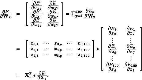
The preceding equation corresponds to line 74 (or so) of rbfn.m:
dE_dW = X1'*dE_dX2;
For derivatives of Ep with respect to x3, we have

Similarly, we have
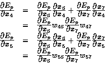
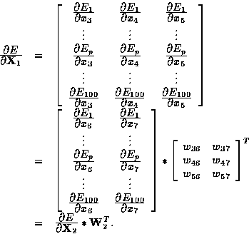
The preceding three equations can be put into matrix form:
![\begin{displaymath}
\begin{array}
{rcl}
\left[
\frac{\textstyle \partial E_p}{\...
...& w_{36}\\ w_{45} & w_{46}\\ \end{array}\right]^T\\ \end{array}\end{displaymath}](img35.gif)
Hence the accumulated derivatives of E with respect to ![]() are
are
rbfn.m:
dE_dX1 = dE_dX2*W';
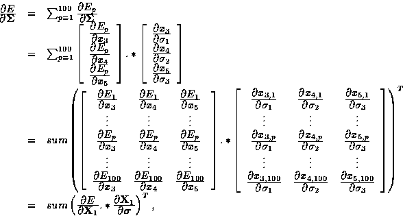
The derivative of layer 1's output with respective to the standard deviations are
![]()
![]()
![]()
![]()
![\begin{displaymath}
\begin{array}
{rcl}
\frac{\textstyle d {\bf X}_1}{\textstyle...
... 1}{\textstyle \sigma_3^3} \\ \end{array}\right]\\ \end{array}\end{displaymath}](img41.gif)
rbfn.m:
dX1_dSigma = X1.*(dist.^2*diag(SIGMA.^(-3)));
The derivative of Ep with respect to the standard deviatins are
![\begin{displaymath}
\frac{\textstyle \partial E_p}{\textstyle \partial \mbox{\bo...
...partial x_5}{\textstyle \partial \sigma_3}\\ \end{array}\right]\end{displaymath}](img42.gif)
 |
(1) |
rbfn.m:
dE_dSigma = sum(dE_dX1.*dX1_dSigma)';
Now we are moving toward the final step: to calculate the derivative
of E with respect to the centers of the gaussians.
Since
 , the derivative
of x3 with respect to
 ![]() are
are

![]()
![\begin{displaymath}
\begin{array}
{rcl}
\left[
\begin{array}
{cc}
\frac{\textsty...
...x_5 \\ \end{array}\right]
\right)
*
{\bf C}
\right\}\end{array}\end{displaymath}](img48.gif)
![\begin{displaymath}
\begin{array}
{rcl}
\frac{\textstyle \partial E}{\textstyle ...
...,p} \\ \end{array}\right]
\right)
*
{\bf C}
\right\}\end{array}\end{displaymath}](img49.gif) |
(2) |
The first term in the curly braces can be further simplified:


The preceding equation corresponds to line 81 (or so) of rbfn.m:
dE_dCenter=diag(SIGMA.^(-2))*((dE_dX1.*X1)'*X0-diag(sum(dE_dX1.*X1))*CENTER);