CS5652: Artificial Neural Networks
Implementation of tanmlp.m

  

Figure 1: A 1-3-2 MLP.

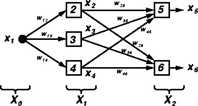
For simplicity, suppose that we are dealing with a 1-3-2 multilayer perceptron with hyperbolic tangent activation functions, and we have 100 input-output data pairs as the training data set. The training data set can be represented by a $100 \times 3$ matrix:

$$\left[ \begin{array} {ccc} x_{1,1} & t_{5,1} & t_{6,1} \\ \v... ...dots \\ x_{1,100} & t_{5,100} & t_{6,100} \\ \end{array}\right]$$

where the input part is denoted by ${\bf X}_0$:

$${\bf X}_0 = \left[ \begin{array} {ccc} x_{1,1} \\ \vdots \\ x_{1,p} \\ \vdots \\ x_{1,100} \\ \end{array}\right]$$

and the output (target) part is denoted by ${\bf T}$:

$${\bf T}= \left[ \begin{array} {cc} t_{5,1} & t_{6,1} \\ \vdo... ... \vdots & \vdots \\ t_{5,100} & t_{6,100} \\ \end{array}\right]$$

For discussion convenience, we shall also defined ${\bf X}_1$ and ${\bf X}_2$as the node outputs for layer 1 and 2, respectively:

$${\bf X}_1 = \left[ \begin{array} {ccc} x_{2,1} & x_{3,1} & ... ...dots \\ x_{2,100} & x_{3,100} & x_{4,100} \\ \end{array}\right]$$

$${\bf X}_2 = \left[ \begin{array} {cc} x_{5,1} & x_{6,1} \\ ... ... \vdots & \vdots \\ x_{5,100} & x_{6,100} \\ \end{array}\right]$$

Similarly, the parameters ${\bf W}_1$ and ${\bf W}_2$ for the first and second layers can be defined as follows:

$${\bf W}_1 = \left[ \begin{array} {ccc} w_{12} & w_{13} & w_{14} \\ w_{2} & w_{3} & w_{4} \\ \end{array}\right]$$

$${\bf W}_2 = \left[ \begin{array} {cc} w_{25} & w_{26} \\ ... ... \\ w_{45} & w_{46} \\ w_{5} & w_{6} \\ \end{array}\right]$$

The equations for computing the output of the first layer are

$$\begin{array} {rcl} x_2 & = & tanh(x_1 w_{12} + w_2)\\ x_3 &... ... w_{13} + w_3)\\ x_4 & = & tanh(x_1 w_{14} + w_4)\\ \end{array}$$

or equivalently,

$$\left[ \begin{array} {ccc} x_2 & x_3 & x_4 \\ \end{array}\ri... ... w_{14} \\ w_{2} & w_{3} & w_{4} \\ \end{array}\right] \right).$$

After plugging 100 inputs into the preceding equation, we have

$$\left[ \begin{array} {ccc} x_{2,1} & x_{3,1} & x_{4,1} \\ \v... ... w_{14} \\ w_{2} & w_{3} & w_{4} \\ \end{array}\right] \right),$$

or equivalently,

$${\bf X}_1 = tanh([{\bf X}_0, one]*{\bf W}_1).$$

The preceding equation corresponds to line 47 of tanmlp.m:

X1 = tanh([X0 one]*W1);

The output of layer 2 can be computed similarly and we have line 48 of tanmlp.m:

X2 = tanh([X1 one]*W2);

The instantaneous error measure for the pth data pair is defined by

E_p = (t_5,p-x_5,p)² + (t_6,p-x_6,p)²,

where t_5,p and t_6,p are the pth target outputs; x_5,p and x_6,p are the pth network outputs. The derivative of the above instantaneous error measure with respect to the network outputs is written as

$$\frac{\textstyle \partial E_p}{\textstyle \partial {\bf X}_2... ...t_{5,p} - x_{5,p}) & -2(t_{6,p} - x_{6,p})\\ \end{array}\right]$$

We can stack the above equation for each p to obtain the following matrix expression:

$$\begin{array} {rcl} \frac{\textstyle \partial E}{\textstyle ... ...nd{array} \right] \right) = -2 ({\bf T}- {\bf X}_2),\end{array}$$

where ${\bf X}_2$ is the actual output of the MLP. The preceding equation corresponds to line 59 of tanmlp.m:

dE_dX2 = -2*(T - X2);

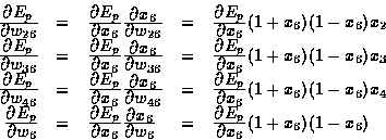
Now we can compute the derivatives of E_p with respect to the second-layer's weights and bias. The derivatives of E_p with respect to the parameters (weights and bias) of node 5 are

$$\begin{array} {rllll} \frac{\textstyle \partial E_p}{\textst... ...ial E_p}{\textstyle \partial x_5} (1+x_5)(1-x_5) \\ \end{array}$$

The derivatives of E_p with respect to the parameters (weights and bias) of node 6 are

$$\begin{array} {rllll} \frac{\textstyle \partial E_p}{\textst... ...ial E_p}{\textstyle \partial x_6} (1+x_6)(1-x_6) \\ \end{array}$$

We can combine the above eight equations to have the following concise expression:

$$\frac{\textstyle \partial E_p}{\textstyle \partial {\bf W}_2... ... E_p}{\textstyle \partial x_6}(1-x_6)(1+x_6)\end{array}\right].$$

Therefore the accumulated gradient vector is  

$$\begin{array} {rcl} \frac{\textstyle \partial E}{\textstyle ... ... {\bf X}_2}.*(1+{\bf X}_2).*(1-{\bf X}_2) \right]\\ \end{array}$$ (1)

The preceding equation corresponds to line 60 of tanmlp.m:

dE_dW2 = [X1 one]'*(dE_dX2.*(1+X2).*(1-X2));

For derivatives of E_p with respect to x₂, we have

$$\begin{array} {rcl} \frac{\textstyle \partial E_p}{\textstyl... ...E_p}{\textstyle \partial x_6} (1-x_6)(1+x_6)w_{26}.\end{array}$$

Similarly, we have

$$\begin{array} {rcl} \frac{\textstyle \partial E_p}{\textstyl... ...E_p}{\textstyle \partial x_6} (1-x_6)(1+x_6)w_{46}.\end{array}$$

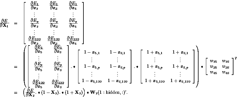
The preceding three equations can be put into matrix form:

$$\begin{array} {rcl} \left[ \frac{\textstyle \partial E_p}{\... ...& w_{36}\\ w_{45} & w_{46}\\ \end{array}\right]^T\\ \end{array}$$

Hence the accumulated derivatives of E with respect to ${\bf X}_1$ are

$$\begin{array} {rcl} \frac{\textstyle \partial E}{\textstyle ... ...f X}_2)\right) * {\bf W}_2 (1:\mbox{hidden}, :)'.\\ \end{array}$$

The preceding equation corresponds to line 62 of tanmlp.m:

dE_dX1 = dE_dX2.*(1-X2).*(1+X2)*W2(1:hidden_n,:)';

By proceeding as what we have done in Equation (1), we have

$$\begin{array} {rcl} \frac{\textstyle \partial E}{\textstyle ... ... {\bf X}_1}.*(1+{\bf X}_1).*(1-{\bf X}_1) \right]\\ \end{array}$$

The preceding equation corresponds to line 63 of tanmlp.m:

dE_dW1 = [X0 one]'*(dE_dX1.*(1+X1).*(1-X1));